Understanding Fuzzy Neural Network using code and animation

In this post we’ll learn about Fuzzy Neural Network, or more specifically Fuzzy Min-Max Classifier. If you don’t know Fuzzy theory, I’ll be briefly going over that too. If you’re already acquainted with the basics of fuzzy sets, you can safely skip that section. In this post, we’ll be talking about a basic fuzzy min-max classifier given by Patrick Simpson in 1992 in this paper.
A] Fuzzy Theory:#
There is always uncertainty in real world experiments. And thus while modeling our systems, we need to take this uncertainty into account. You are already familiar with one form of uncertainty which forms the basis of Probability Theory. Analogous to probability theory, a different way to work with uncertainty was developed by Zadeh known as Fuzzy Set.
A.1] Fuzzy Set vs Crisp Set:#
Before we get into defining fuzzy set and its operations, it is better to understand fuzzy sets in comparison to crisp sets with which you’re already familiar.
We define a set as a collection of elements — e.g A = {x|x ∈ Rand x > 0} where a general universe of discourse is established (in our example, R or set of Real numbers) and each distinct point in that universe is either a part of our set or not.
What we described above is the set theory with which you’re already familiar. Fuzzy sets are also similar to crisp sets but they are more generalized. So crisp sets can be said to be a specific type of fuzzy set.
In crisp set, an element belonging to our universe of discourse is either part of the set or not i.e 0 or 1 but what about the values in between? Can an element be only partially be a part of set?
Let us define the value 0 and 1 as a membership value ( mA(x)) for crisp sets. It is a binary value i.e it can only be 0 or 1 for crisp sets.
For fuzzy sets, this membership value is a continuous value between [0, 1] . In this way fuzzy sets are different from crisp sets. In a fuzzy set, an element’s participation in the set is not strictly defined but it can be a value real between [0, 1] . But what does this mean intuitively?
Fuzzy set allows us to mathematically define ambiguous and subjective terms like ‘young’, ‘many’, ‘few’. We can define a particular value in our universe of discourse as being part of that set with partial participation. Let us take an example to further clarify — Suppose we define a fuzzy set as a set of all ‘young’ people. Then for all people of age [0, 100] we can define a person of age x to have a membership value mA(x) denoting their participation in the set.
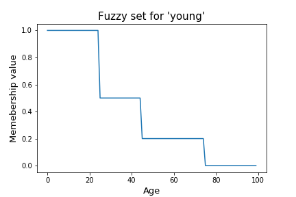
Of course the membership function mA(x) would be different for other people. The above graph shows my interpretation of the word ‘young’ and its meaning.
Thus a fuzzy set is defined as the ordered pair — A = {x, mA(x)} . I’ll also include the full standard definition for good measure.
Let X be a space of points (objects), with a generic element of X denoted by x. [X is often referred to as the universe of discourse.] A fuzzy set (class) A in X is characterized by a membership (characteristic) function m~(x) which associates with each point in X a real number in the interval [0, 1], with the value of m~(x) representing the “grade of membership” of x in A. Thus, the nearer the value of ~A(z) to unity, the higher the grade of membership of z in A.
A.2] Fuzzy set operations:#
Assuming X to be the universe of discourse, A ∈ X and B ∈ X, the fuzzy set operations are defined as follows:
a_. Comparison (Is A = B?)_: iff mA(x) = mB(x) for all x in X
b. Containment (Is A ⊂ B?): iff mA(x) < mB(x) for all x in X
c. Union: m(A ∨B)(x) = max(mA(x), mB(x)) for all x in X
d. Intersection: m(A ∧ B)(x) = min(mA(x), mB(x)) for all x in X
These basic operations are pretty much self explanatory from their definition. So we’ll move on to the meat of the post — the classifier.
B] Fuzzy Min Max Classifier:#
We’ll take a look at this classifier in two different ways. The way this classifier is used to infer the class of a test pattern and the way this classifier neural network is trained i.e inference and learning algorithm.
B.1] Inference:#
Press enter or click to view image in full size
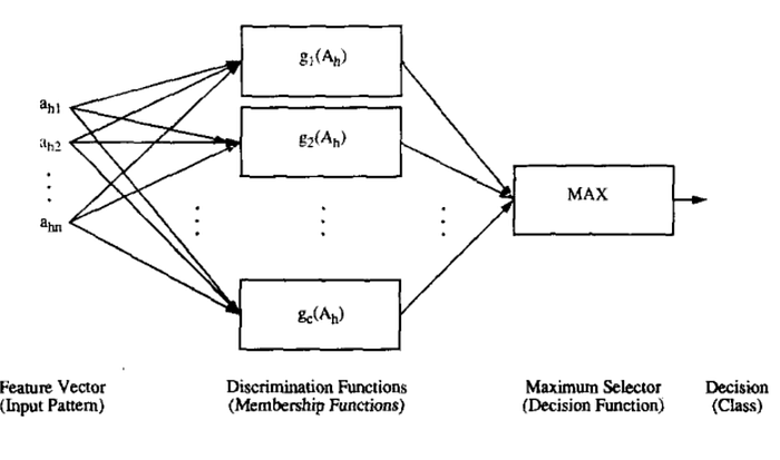
Consider that we have an n-dimensional pattern Ah. And we have K number of discriminant functions where each discriminant function tells the class of the pattern with a confidence score between [0, 1] . We believe the most confident discriminant in our inference i.e the function giving maximum value, we will consider the pattern belongs to that class.
Now just replace the discriminant function with the membership function and you’ll immediately understand how fuzzy sets can be used for class inference. Let the K discriminant functions be K fuzzy sets each defining the participation of the pattern in a specific class. Thus we will believe the pattern belongs to a class defined by the fuzzy set for which the pattern gives maximum membership value.
Hyperbox:
Now before we fit this inference framework in a neural network, we need to understand one alternative representation for the fuzzy set. Consider a 2D universe of discourse [0, 1] . We define a rectangle as a fuzzy set such that all the points within that box have a membership value 1.
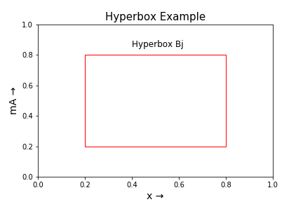
A box is defined by its maximum point and its minimum point. The box shown in the above graph is defined by min-pt V = [0.2, 0.2] and max-pt W = [0.8, 0.8] . This box is also a fuzzy set. And the membership value of this fuzzy set is defined such that all points inside that box have mA(x) = 1 .
But what about the membership value for the points outside the box? The membership value of any point outside the box decreases (< 1) as the distance between that box and the point increases. This distance is averaged over all dimensions (in this case only 2). The membership value for such a definition of box fuzzy set is given by—
Press enter or click to view image in full size
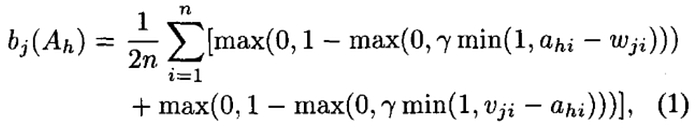
Here Ah is our n-dimensional (in our example 2D) pattern and the box Bj is also defined in n-dimensions (i.e 2 in our case). The above equation is self explanatory except for that γ which is a hyperparameter known as sensitivity or rate of decrease that can be used to control the membership value.
Architecture:
Press enter or click to view image in full size
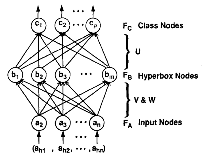
In the neural network architecture shown above, the input nodes are placeholders for the n-dimensional input pattern. There are n input nodes for n-dimensional input space.
The next layer contains Hyperbox nodes. Each hyperbox node is defined by its min-pt and max-pt in n-dimensional space. And each hyperbox belongs to some class.
The final layer contains the class nodes. The number of nodes in this layer is equal to the number of possible classes. In the inference part of the classifier we use the output of these class nodes as the discriminant functions and the class node giving the maximum score is assumed to predict the class value of the pattern.
One important detail that needs to be understood is the interaction between class node layer and hyperbox layer. I said that each hyperbox (node) belongs to some class. When considering the class node output, we consider the maximum membership value among the hyperboxes belonging to that class. The membership values given by the hyperboxes belonging to other classes are not considered.
E.g Suppose hyperboxes Bj and Bk belong to class 1 and hyperbox Bl belongs to class 2 (we only have three hyperboxes in our classifier). And we have two class nodes C1 and C2. For a pattern Ah the hyperboxes give membership values as [0.4, 0.8, 0.7] respectively.
To calculate the output of the class node C1 — C1 = max([0.4, 0.8, 0.0]) = 0.8 . We consider that the link between Bl and C1 node represents 0 and links between Bj and Bk represent 1. Hence their contribution in defining the class node value.
Similarly for class node C2 — C2 = max([0.0, 0.0, 0.7]) = 0.7 . Now we have [C1, C2] = [0.8, 0.7] . To predict the class, we take the class with the maximum score. Therefore pattern Ah belongs to class 1.
B.2] Learning Algorithm:#
A very natural question might have arisen in your mind after going through the above section. How do we get these hyperboxes? Once we have the hyperboxes, we can use the above described method to the predict the class of the patterns. But first we need an algorithm to learn these hyperboxes based on the data we have available.
The learning algorithm is also pretty straightforward. I would recommend that you also go through the learning algorithm described in the original paper to further cement your understanding.
Recall that the hyperbox is defined using two pts - min-pt and max-pt (notation-wise Vj and Wj for j-th hyperbox). When we begin our training, we have no learned hyperboxes i.e 0 hyperbox nodes in our network. As we observe the patterns in the training set one by one, we’ll start creating these nodes.
The learning algorithm can be categorised into two distinct phases — Expansion phase and Contraction phase.
a. Expansion Phase:
Let Xh be an n-dimensional training pattern belonging to class Y. The first thing we do is find the most suitable hyperbox for expansion. We take all the hyperboxes belonging to the class Y and calculate their membership values. The hyperbox with the maximum membership value is the most suitable candidate for expansion.
Let Bj be the hyperbox most suitable for expansion. Before we expand, we need to meet the expansion criterion which is a condition defined by—
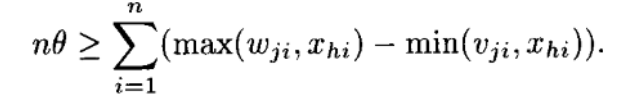
where θ is a hyperparameter known as the expansion bound. This hyperparameter controls the maximum expansion allowed for a hyperbox.
If our hyperbox satisfies the above condition then the hyperbox is expanded as follows —
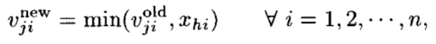

where Vj and Wj are the new min-pt and max-pt of the hyperbox Bj. Intuitively, the hyperbox expands such that the training point Xh is included in its region.
But what happens if the Bj hyperbox does not satisfy the expansion criterion? In that case, we move to the next most suitable hyperbox defined by the descending order of the membership values and check the expansion criteria for that box. And we do so until we a find a suitable box or we run out of boxes. In the latter case that we can find no suitable hyperbox for expansion, we create a new hyperbox for class Y with Vj (min-pt) = Wj (max-pt) = Xh .
But we’re not done yet, what if two hyperboxes overlap each other? If they belong to the same class then the classifier will correctly predict the class but if two hyperboxes from different classes overlap, then the classifier will predict that a pattern belongs to both the classes. We definitely want to avoid this situation. Let’s see what can be done to avoid this kind of overlapping.
b. Contraction Phase:
I’ll first briefly describe the phase and then give the actual conditions that define the operations we need to perform on our hyperbox.
Suppose from the last phase that we found a suitable hyperbox meeting the expansion criteria and we expanded the box Bj. We need to make sure that this expanded box does not overlap with another hyperbox belonging to a different class. Overlap between hyperboxes of same class is allowed, so we’ll only check for overlap between expanded box and hyperboxes of different classes.
While checking for overlap between the expanded hyperbox (Vj, Wj) and a test box (Vk, Wk), we measure the overlap between them in all the n-dimensions i.e we check for overlap in every dimension and at the same time we also note down the value of that overlap (how much overlap is there?). Thus we can find the dimension among the n-dimensions in which the overlap is minimum. We note down this dimension and this overlap value. If we find that the boxes do not overlap in any dimension, then we ignore this box and move to the next test box.
Press enter or click to view image in full size
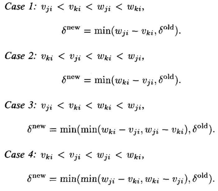
We calculate the 𝛿new value for each dimension according to the above cases (which cover all possible ways of overlap). Out of these overlap values, we find the dimension Δ in which this overlap (𝛿new) is minimum. In the original paper, this mechanism is explained in the context of implementing it in a program. But as long as you understand what is happening, you can implement the logic differently to get the same result.
Now we have the dimension in which there is minimum overlap (Δ) between two boxes. Our goal is to contract the expanded box Bj but we want the contraction to be as small as possible while still removing the overlap. So we’ll use the dimension with minimum overlap (Δ) and contract our box in that dimension only.
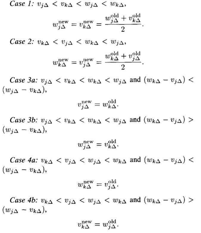
Based on the kind of overlap in the Δth dimension, we contract the box Bj in that dimension using the above given cases.
Thus we have expanded a hyperbox and tested it for overlap against different class hyperboxes. And in cases of overlap, we have searched for a way to contract the box minimally and removing the overlap.
c. Example:
We’ll go through a toy example to make sure that we clearly understand what is happening.
Suppose we have 4 patterns in our training set as follow —
patterns: A1 = [0.2, 0.2] A2 = [0.6, 0.6] A3 = [0.5, 0.5] A4 = [0.4, 0.4]class: d1 = 1 d2 = 2 d3 = 1 d4 = 1
We’ll take a pattern one-by-one and visually inspect the result of the learning algorithm.
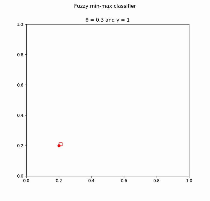
Pattern: [0.2, 0.2] Class: 1 No suitable hyperbox found for expansion. Add a new hyperbox of class 1 with Vj = Wj = [0.2, 0.2]
Press enter or click to view image in full size
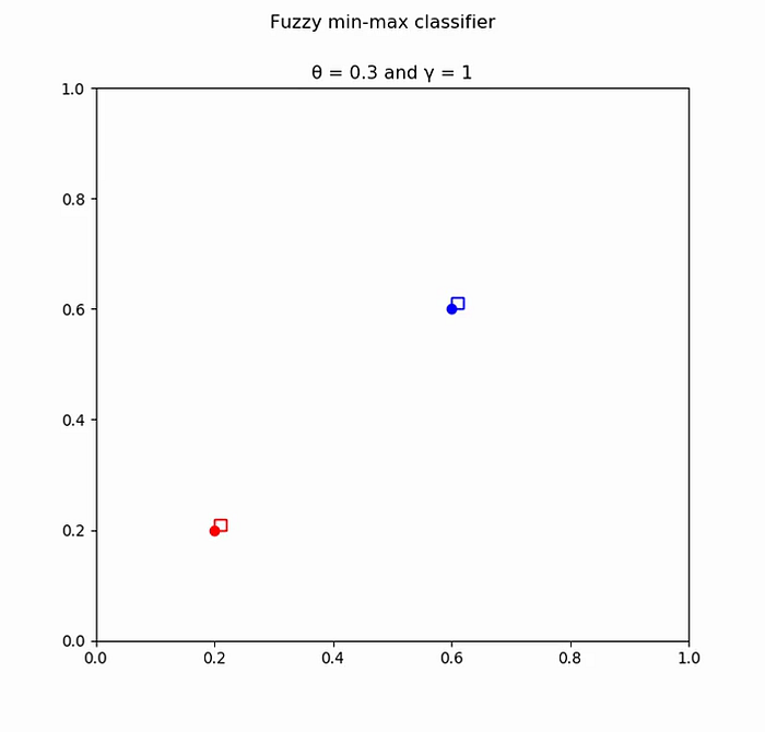
Pattern: [0.6, 0.6] Class: 2 No suitable hyperbox found for expansion. Add a new hyperbox of class 2 with Vj = Wj = [0.6, 0.6]
Press enter or click to view image in full size
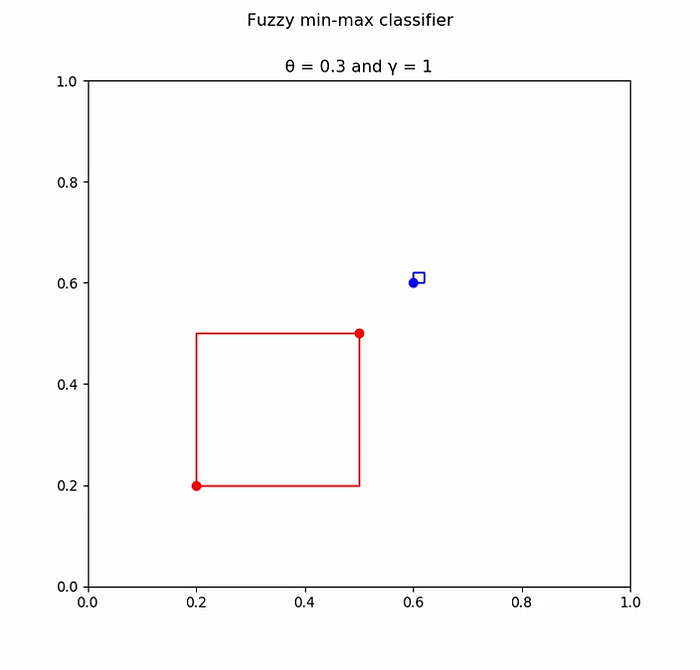
Pattern: [0.5, 0.5] Class: 1 Most suitable hyperbox: Vj = [0.2, 0.2] Wj = [0.2, 0.2] Expansion criteria satisfied. Hyperbox expanded. New hyperbox: Vj = [0.2, 0.2] Wj = [0.5, 0.5] No overlap found.
Press enter or click to view image in full size
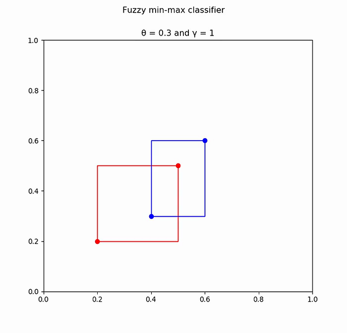
Pattern: [0.4, 0.3] Class: 2 Most suitable hyperbox: Vj = [0.6, 0.6] Wj = [0.6, 0.6] Expansion criteria satisfied. Hyperbox expanded. New hyperbox: Vj = [0.4, 0.3] Wj = [0.6, 0.6] Overlap with class 1 hyperbox found.
Press enter or click to view image in full size
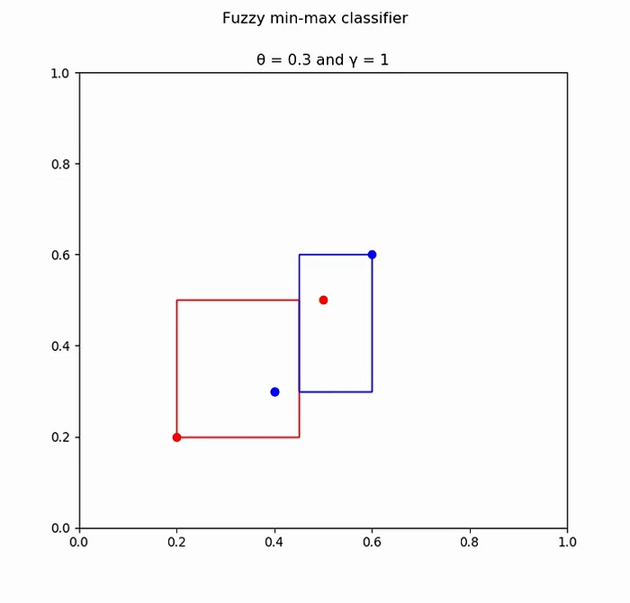
Expanded box: Vj = [0.4, 0.3] Wj = [0.6, 0.6] Test box: Vk = [0.2, 0.2] Wk = [0.5, 0.5] Minimum overlap found in dimension: Δ = 0 (i.e horizontal dimension) Both hyperboxes are adjusted in that dimension to remove overlap. Overlap removed.
Press enter or click to view image in full size
Thus we apply the learning algorithm and derive hyperboxes based on the training data.
Note: The observant among you will have noticed that if we use the hyperboxes learned in the above example and use them to predict the points in the training set, then the classifier will give wrong prediction. That is correct, the above classifier does not have a 100% accuracy (this one only has 50%). What can be done to improve performance?
We have a hyperparameter θ with which we can play around to improve the results. When you use a high value for θ then the maximum allowed size of the hyperboxes increases and this increases the chance that a incorrectly labelled pattern falls in that region.
But if we take too small a value for θ then the number of hyperboxes will increase and overfit the newly added points. This way our classifier loses the ability to generalize well and gives bad performance over points outside its training set.
You need to experiment with different values of θ to find the value that gives the best performance. I will add a couple examples with different values of θ and you can observe yourself how θ affects hyperbox creation.
Example 1:#
Example 2:#
Code:#
You can find all the code for the fuzzy min-max classifier and the animation code on my github.
I encourage you to try coding this classifier on your own to make sure you properly understand every aspect of the algorithm.
Thank you for reading and stay tuned for further posts!